Jacobi Iteration

Jacobi Iteration

In this example we will get very close to a "real" application in numerical fluid mechanics. We will solve the following Poisson in two dimensions

L(u)=(d_xx+d_yy)u=0

on a unit square [0,1]x[0,1] with Dirichlet boundary conditions

u=sin(Pi*x)*exp(-Pi*y) for x=0, x=1, y=0, y=1

Using a Cartesian, uniform mesh and second-order accurate, central finite-differences, the spatial operator is discretized as follows:

L(u)=(u_i+1,j-2u_i,j+u_i-1,j)/dx²+(u_i,j+1-2u_i,j+u_i,j-1)/dy²

for all 1<=i<=m, 1<=j<=n and - for simplicity - dx=dy. Note that the boundaries correspond to the indices i=0,m+1 and j=0,n+1.

The Jacobi method for iteratively solving the above system can be obtained as follows. First, modify the equations by introducing a time-derivative:

d_t u=L(u) -> (uⁿ⁺¹-uⁿ)/dt=L(uⁿ)

We will iterate until d_tu=0, which gives the solution to the original problem. Substituting the discrete spatial operator and taking the maximum stable "time step" gives the formula for the Jacobi iteration:

uⁿ⁺¹_i,j=(u_i+1,jⁿ+u_i-1,jⁿ+u_i,j+1ⁿ+u_i,j-1ⁿ)/4

Note that the right-hand-side consists only of value at the previous time level "n", and, therefore, the formula is explicit. This method is not efficient for practical computations (converges slowly, accumulates round-off) but serves its purpose as an example. An implementation for a single processor is accessible below.

• single-processor code

How to approach the parallelization of the algorithm?

1. Functional decomposition or domain decomposition?
   
   -> there is nothing else to do but to execute the Jacobi formula on a large amount of data many times. Therefore, we will certainly choose a domain decomposition technique.
   
   
2. How to decompose the domain/data?
   
   Look at the algorithm. First observation: the formula is fully explicit per time step. That means that once all required previous values are known, all those values can be updated locally without need for communication. Second observation: the right-hand-side for a given node (i,j) is a function of four neighboring node values (i-1,j), (i+1,j), (i,j-1), (i,j+1). This means that after each time step, we need to communicate a limited amount of data. More specifically: for this type of 3-point difference formulas (in each direction), it is sufficient to communicate one "layer" of data between neighboring processes/processors. In order to minimize the data volume which we need to communicate, it makes sense that each processor deals with contiguous data. In this fashion the "boundary" with neighboring chunks is minimized. Furthermore, it is useful to define "ghost cells" at internal boundaries. These ghost cells duplicate the required additional data layer such that all differencing stencils can be evaluated locally. The communication then consists in up-dating the value of those ghost cells only.
   
   
3. This is a 2D case, should i decompose the data in both directions?
   
   Good question. The answer is: yes. However, in this example we will start with 1D decomposition for simplicity. Let us decompose the second index only.

So, here comes the first task:

• write a routine which decomposes an integer number n into nproc parts as evenly as possible. The routine has two input arguments: scalar integers n, nproc; it has two output arguments: two integer arrays of size nproc, containing - respectively - the first and last index held by a processor 0<=myrank<=nproc-1.

Note: if the pointer arrays are called jbeg, jend, then the local arrays will hold the index range jbeg(myrank)-1:jend(myrank)+1 because of the two "ghost cells". Their dimension will then be jend(myrank)-jbeg(myrank)+2!

• decomposition routine: computation of pointers

So, here comes the second task:

• Modify the sequential version of the jacobi program such that - after the usual MPI initialization phase - every processor computes these pointers. Dimension the locally held arrays correctly. Attention: do you know how much data each processor receives at compile time exactly? We suppose that nproc and the system size n, m is known when compiling. If you do not want to dynamically allocate arrays, a small over-dimensioning is necessary.
  
  Go ahead and modify the assignment of boundary conditions, the jacobi step and the rest of the program such that you operate only on the local bounds of the data.

The result should be a nearly-functional Jacobi program; the only missing part now is the communication step which needs to be performed after each iteration. An example for a driver routine is here:

• driver routine

So, here comes the third task:

• Write a communication subprogram which takes care of the exchange of data between neighboring processors. Input arguments: the local array, the pointers, the rank of the processor, the communicator, the size of the communicator. Output arguments: the array containing updated ghost-cell entries.
  Things to keep in mind:
  • the communication is pair-wise between neighboring processes; each pair exchanges two lines of ghost-cell data; in general each processor has two neighbors, which makes for 4 communication operations per processor - 2 sends and 2 receives.
  • the available communication methods are either MPI_SEND and MPI_RECV or MPI_ISEND and MPI_IRECV or MPI_SENDRECV (which we have not treated before). Watch the order!
  • the "end processors" do not have 2 neighbors!
  • ...

Possible solutions (of different quality!) are contained in the following link:

• several variants of communication subroutines
• another variant in C

Some hints for debugging the program:

• Did you forget one of the "five essentials" of an MPI program?
  
  include "mpif.h"
  call MPI_INIT(ierr)
  call call MPI_COMM_RANK(MPI_COMM_WORLD,myrank,ierr)
  call MPI_COMM_SIZE(MPI_COMM_WORLD,nprocs,ierr)
  call MPI_FINALIZE(ierr)
  
  
• Did you forget to declare the status array wherever you call MPI_RECV?
  
  integer istat(MPI_STATUS_SIZE)
  
  
• Did you correctly declare the local arrays and use the pointers jbeg, jend consistently for transferring local to global indices?
• A common mistake is forgetting that the processor rank varies between 0 and nprocs-1 (and NOT 1 to nprocs).
• Include write statements. Most problems are due to the fact that some information is not known to all processors or mixed up. You will see many bugs immediately.
• Run parts of the code; the full code is probably more difficult to debug.
• Check iterative convergence & convergence with number of modes (should be second order).
• Plot the result & compare to exact solution; often you will see where in the domain things do not work. How do you write a distributed array to a single file? The practical way is to let one "i/o master" process (e.g. myrank=0) receive and write data to file, while all oters send their data to this master. Attention: does the received data always fit into the master's local buffer?

Finally, we want to know which is the most efficient method of communication (supposing that the rest of the code will be more or less equivalent for all). You can obtain timing information by using the MPI_WTIME function as follows:

t0=MPI_WTIME()
some code
t1=MPI_WTIME()
if(myrank.eq.0)write(*,*)'elapsed time: ',t2-t1

which will give the elapsed time in seconds. Strictly, the maximum over all elapsed times should be computed, using e.g. MPI_REDUCE. Also: for timing purposes you should not run all virtual processes on the master node, but instead use the available ressources. If you simply execute

mpirun -np <no. of procs> <executable>

the script mpirun will decide where your processes are sent. You can also force the selection by:

mpirun -np <no. of procs> -machinefile <file> <executable>

where <file> is the name of a file containing a list of nodes (one per line) where processes should go, e.g.:

lince01.ciemat.es
lince02.ciemat.es
lince03.ciemat.es
lince04.ciemat.es

sends processes (in order) to nodes 01, 02, 03, 04. You can repeat nodes in this file with the result that more than one process is executed on that node.

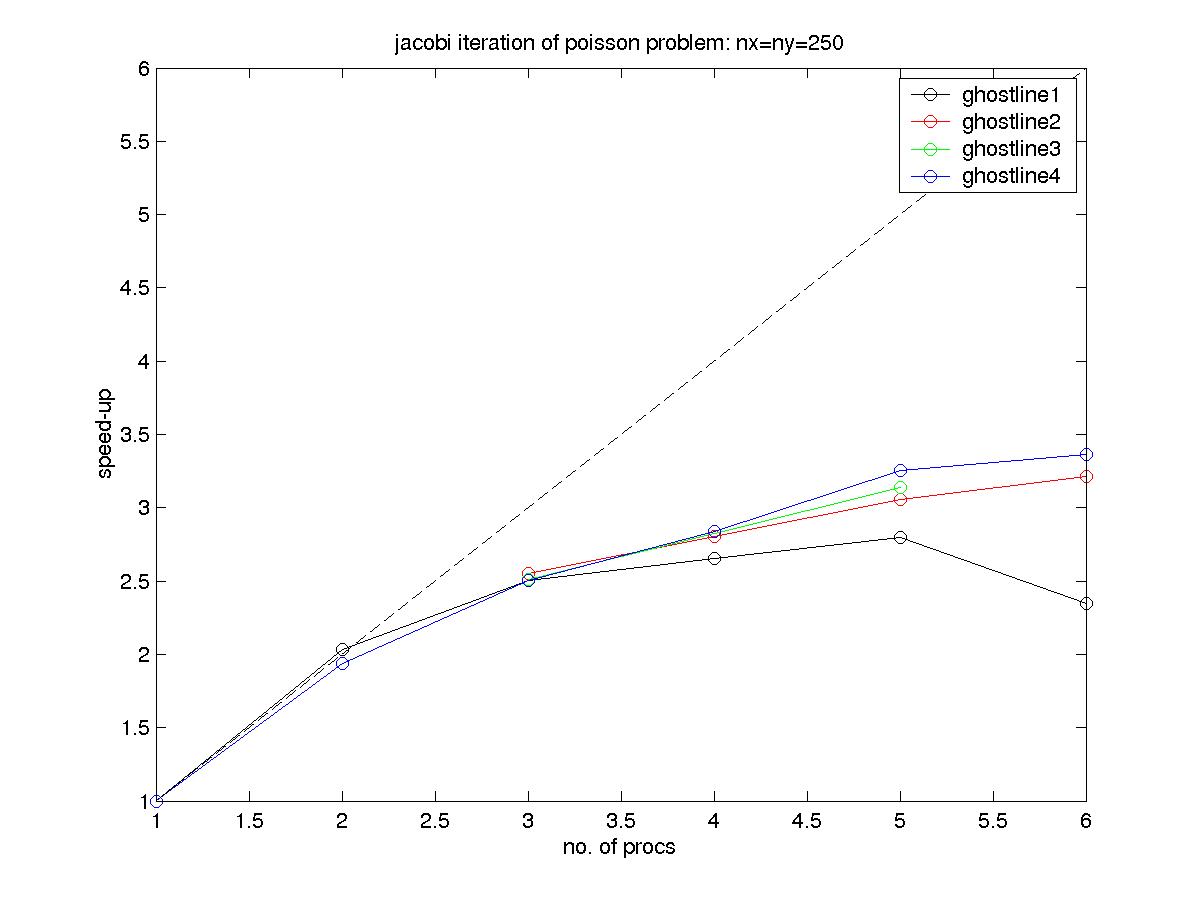
Results of timing the example solution - using the 4 different suplied communication routines - on fenix.ciemat.es are plotted in this graph (eps) (jpg)(tiff). You can see that the ordering of the communication makes a difference! By the way, relative parallel speed-up is measured as follows:

S=T₁/T_p

where T₁ is the execution time using one processor and T_p the corresponding time for p processors. The other useful measure of performance is parallel efficiency, computed as follows:

E=T₁/(p*T_p)

Here, again all necessary routines to run the sequential and parallel program are available for convenience:

• single-processor code
• README for parallel version
• parallel driver routine
• communication subroutines 1 2
• makefile example
• definition of real types

Jacobi Iteration