


Contents
 |  |  | 2.2 Analytic solution to Riemann's problem | Contents | Index |
Let us consider the initial-value problem with the following data
In our case, both characteristic fields are genuinely non-linear (GNL), since [5]
This fact signifies that the two wave-fields can either be smooth solutions called simple waves ("rarefactions" in the terminology of gas dynamics) or (discontinous) shocks. In general it exists one more possible type of solution, that of a contact discontinuity, which however does not appear in the present one-dimensional case but is encountered when carrying both velocity components in the equations (cf. section ).
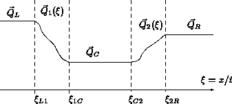
Zones and limiting coordinates of the solution to the Riemann problem for t>0.
The solution to the problem will consist of constant states separated by either shock waves or rarefaction waves. The solution for t>0 can be divided into zones as shown in figure. Zones "1" and "2" have zero width in the case of a respective shock and will otherwise consist of a smooth variation over a finite interval.
We begin by studying shock waves. The notion of a weak solution of a conservation law has been coined by Lax [6] and is explained in § 4. A volume integral balance across a discontinuity propagating at speed sigma gives for our system (square brackets denoting a jump)
such that we get explicitly
The mathematical solution for a jump between left and right states Ql, Qr satisfying xl<xr is the following
where the ratio z=hr/hl is a paramter. Next we need to select the physically meaningful sign of the velocity jump in the mathematical expression. From the shock conditions first derived by Lax [6] (also called "entropy conditions" with respect to gas dynamics) we know that the following inequalities hold for 1-shocks
By substitution of the jump conditions one can verify that these inequalities can only be satisfied when z>0 and the - sign is selected in the jump conditions in the case of a 1-shock. Moreover, sigma is seen to be negative and the inequalities sigma<ur, sigma<ul hold. We thus have the situation shown in figure. The flow constantly feeds characteristic waves into the back of the shock while no information on the shock preceeds its own propagation. The fact that z>0 shows a shock to be "compressive", i.e. that our height variable h always increases when a shock has passed. Finally, the bounds on sigma prove that fluid particles pass a 1-shock from left to right.
The case of a 2-shock is analogous: we obtain z<1 and need to select the + sign in the jump conditions.
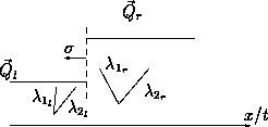
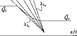
Schematic of (a) a 1-shock and (b) a 1-rarefaction wave.
Let us now turn to the rarefaction curves. These are so-called simple waves, i.e. regions of the solution in which the variables vary smoothly between two states. Since the k-characteristic speed always increases through a k-rarefaction curve (lambdak(Q(x/t) increases as x/t increases) the k-characteristic paths do not cross and form what is sometimes called an expansion fan ( figure). One has thus in a 1-rarefaction wave:
Associated to each k-simple wave there are (n-1) k-Riemann invariants IRk that satisfy
and which remain constant within the interval covered by the k-simple wave. In our case (of an n=2 dimensional system of equations), it can be verified that the following expressions are the two Riemann invariants:
With respect to the 1-rarefaction curve, we thus have
Using equation and equation we can conclude that 1>=(hr/hl)>0, i.e. that the water height decreases in a rarefaction wave. Again, the situation is analogous in the case of a 2-rarefaction (lambda2(Qr)>=lambda2(Ql) and 1>=(hl/hr)>0). We can now introduce a dimensionless parameter chi= -log(hr/hl)>=0 (chi=log(hr/hl)>=0 for a 2-rarefaction) such that the rarefaction curves can be described by the following formulas:
Similarly, the shock curves can be parmetrized using chi=-log(z)<=0 for the 1-shock and chi=log(z)<=0 for the 2-shock, viz.
With these ingredients it is now possible to put together the one-parameter functions associated with each "family" of curves, i.e. for each wave field whatever its type might be:
The global solution to the Riemann problem is obtained by defining a set of transformations across each field in order to connect the left and right initial states. Before proceeding, we need the following three properties:
Particularly, the first inequality can be verified by considering that the drivative f'1 is monotone in both the positive and negative branch of chi.
Defining the vector of primitive variables V=(h,u)=(v1,v2), we introduce now the general transformations Tchii, i=1,2:

Solving the Riemann problem comes down to determining the real numbers chi1 and chi2 for which:
Explicitly, the transformation given above can be written as:
It is useful to define the global parameters
From the first component of the above formula we deduce
while we get from the second component
Using the property and relation, we rewrite this as
We can now: (i) find bounds on the admissiblility of the initial data and (ii) formulate criteria for the appearance of either rarefactions or shock curves in the solution depending on the initial data. To this end let us consider the rarefaction curves which present the critical part of the solution.
Suppose that the 1-family is a rarefaction curve, i.e. chi1>=0. In the limit between a shock/rarefaction chi1=0 and from the formula we have C=f1(log(B))sqrtB. Since we know that f'1>0, we find that
for the 1-family to be a rarefaction curve. The solution of the previous formula in this case can be given explicitly, viz.
from which arises as a further condition
for chi1 to be real. If this condition is violated no real chi1 exists and in fact a dry zone develops on the back side of the rarefaction. In that case, the velocity is not defined and we will arbitrarily set it to zero.
Looking at the 2-family, we obtain from formula and using the formula:
for the 2-family to be a simple wave. In that case the solution is
from which the admissibility criterion (beyond which a dry zone occurs):
as in the previous case. Note that the solution for the shock curves (i.e. chi1 and/or chi2 negative) is an implicit function for the chi's that has to be solved numerically. However, a solution of the shock curve is only necessary in the case that both families are shock curves since otherwise the problem is entirely defined by specifying the central state from the rarefaction relations and the variation across the shock is consistently obtained. More specifically, in the mentioned case of a double shock solution - returning to the height ratio z1 as the unknown parameter - we can choose to solve the following formula that applies to the 1-shock:
by using a Newton iteration, say. With respect to admissibility, the shock curves do not introduce any further limitation on the initial data. We can now conclude:
otherwise a dry zone develops in between the initial states. The 1-family of waves is a simple wave if
and otherwise a shock wave. The 2-family is a simple wave if
and otherwise a shock wave (C and B are defined in equations).
In practice, one of the following four configurations can arise:
which we can now decide from the initial data by applying the criterion and the criterion. The central state QC can thus be deduced from equation in cases (i)-(ii) and from equation in case (iii) while iterating the equation is necessary in case (iv). What is now left to do in order to terminate the solution is the determination of the limit coordinates of the zones "1" and "2" ( figure) and the explicit variation of variables through the rarefaction curves.
We first remark that the solution to the Riemann problem is completely self-similar with xi=x/t as the similarity variable and as such it can be expressed conveniently in one-dimensional xi-space. In the case of a 1-shock (2-shock) the position of the discontinuity xiL1=xi1C (xiC2=xi2R) is equal to the shock speed sigma given by relation. Throughout the region covered by a k-rarefaction curve, we know that the solution is constant along characteristic curves dx/dt=lambdak and that these characteristics are straight lines, i.e. dx/dt=xi. Moreover, we know about the constancy of the associated k-Riemann invariant IRk. Together we obtain:
The zone limits are obtained by calculating the propagation speeds of the bounding characteristics:
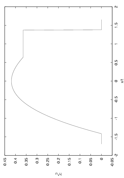
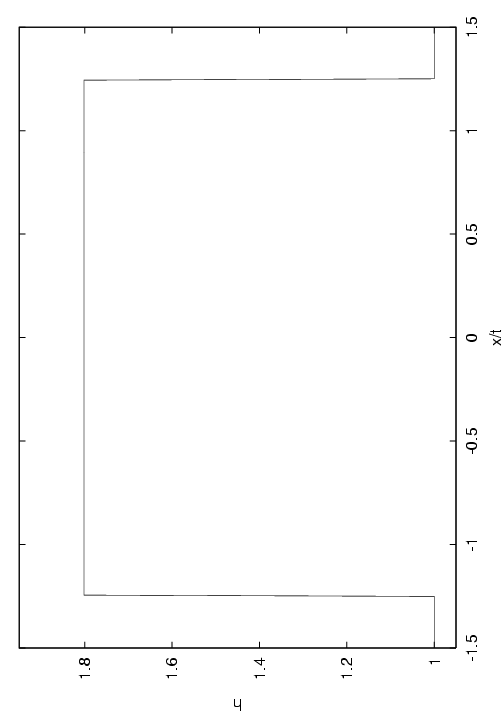
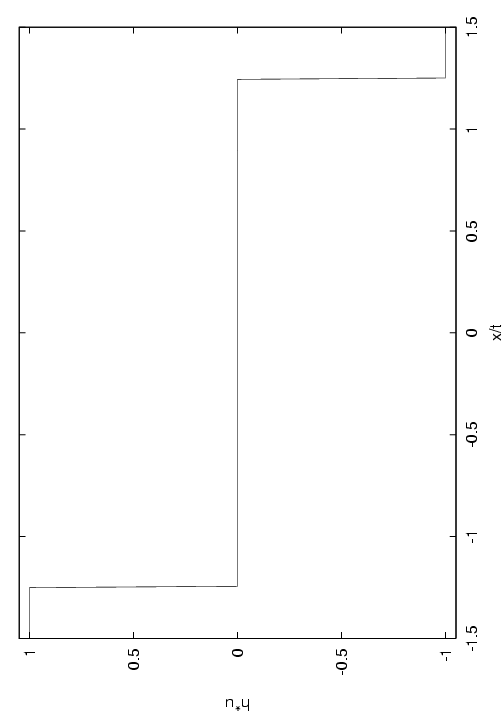
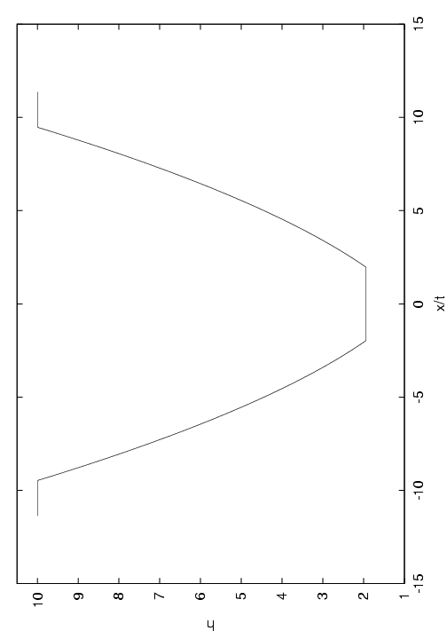
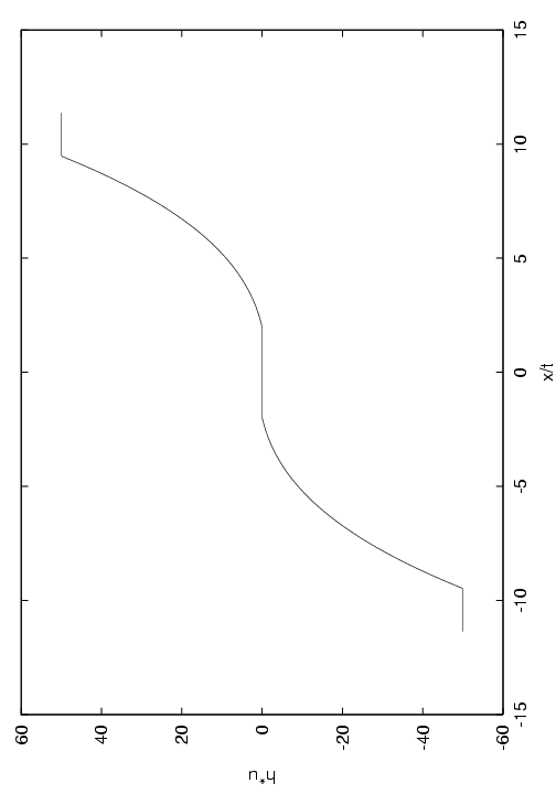
This completes the solution of the Riemann problem. An explicit algorithm is given in appendix 5. Some examples for different initial data are shown in figure.
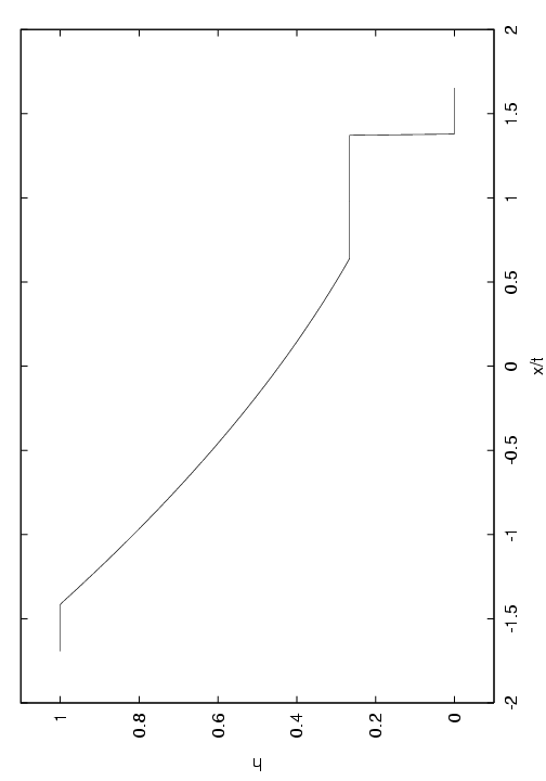
(b)
(c)
markus.uhlmann AT ciemat.es
 |  |  | 2.2 Analytic solution to Riemann's problem | Contents | Index |